The RL circuit

Inductance, current continuity and an exact reference for numerical models.

A winding as an equivalent circuit

A first approximation to a winding is a series resistance R and inductance L. Resistance represents conductor loss; inductance stores magnetic energy. With a stationary rotor, rotational back EMF is zero, so this circuit isolates electrical dynamics.

At the instant a constant voltage is applied to an unenergized winding, current is zero and all the voltage appears across L. As current rises, Ri grows and the current derivative falls.

Exact switch-on response

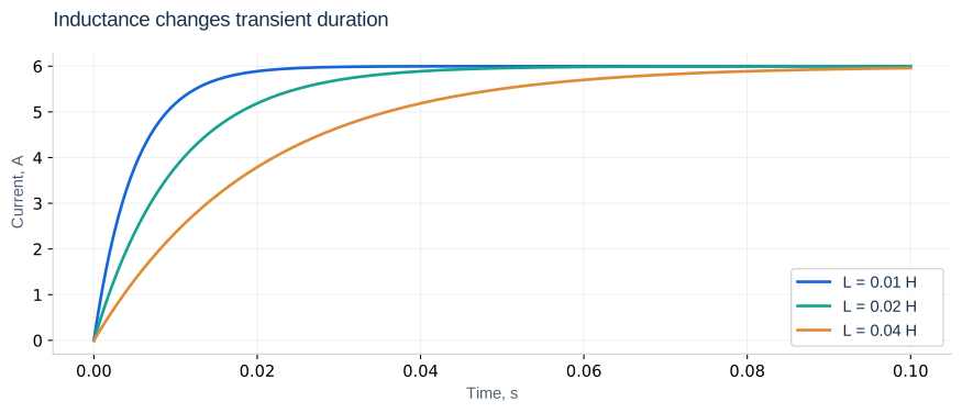
For U = 12 V, R = 2 Ω and L = 0.02 H, τe = 0.01 s and final current is 6 A. Initial slope is 600 A/s. Current is about 3.79 A at 10 ms and 5.96 A at 50 ms. Increasing L changes the transient duration but not the final DC current. R changes both. Always identify the parameter being varied and what is held constant.

Current decay requires a closed path

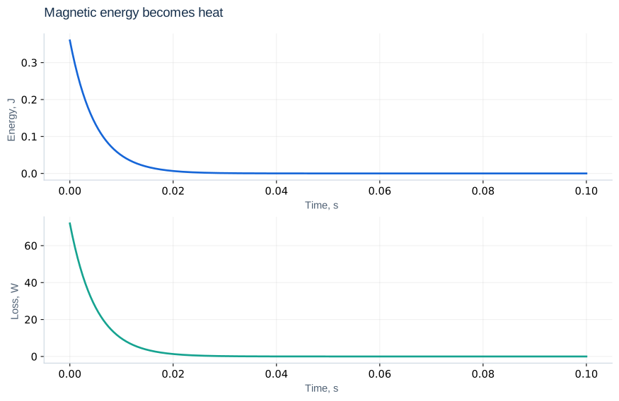
Replacing the voltage source with a short circuit leaves a closed RL loop. With u = 0, i = i₀ exp(−t/τe), and magnetic energy becomes heat. Opening the circuit is different: a diode, arc, parasitic capacitance or protective circuit must provide a path. Instantaneously forcing inductor current to zero while requiring finite voltage is inconsistent.

Energy as an independent check

Input power supplies loss and changing stored energy. With u = 0, energy decreases at Ri². At 6 A and L = 0.02 H, the initial energy is 0.36 J; the integrated loss over a sufficiently long decay should approach that value. A wrong resistance sign can create an artificial growing response.

Numerical experiment

import numpy as np
from scipy.integrate import solve_ivp
R, L, U = 2.0, 0.02, 12.0
t = np.linspace(0, 0.08, 801)
sol = solve_ivp(lambda t, y: [(U-R*y[0])/L],
                (t[0], t[-1]), [0.0], t_eval=t,
                rtol=1e-8, atol=1e-10)
assert sol.success, sol.message
exact = U/R * (1-np.exp(-R*t/L))
print(np.max(np.abs(sol.y[0]-exact)))

Compare both solutions at identical times; the difference is in amperes. If tighter tolerances do not improve it, check the reference formula, parameters and initial conditions.

Directions and the switching procedure

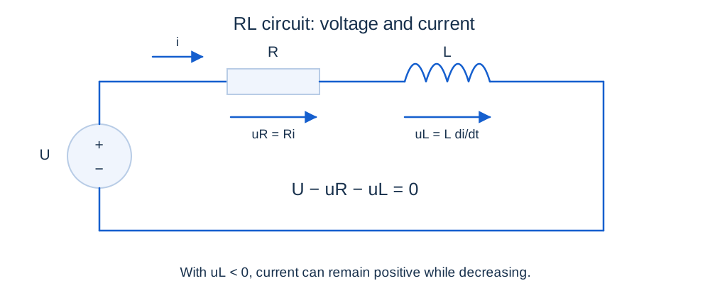
Choose a reference direction for current and voltage drops. Reversing the source changes U, not the chosen direction of i; a negative solution means actual current flows against the arrow. Find i₀ from the old circuit and i∞ from the new DC circuit. The resistance seen by the inductor determines τ = L/Req. Suppress independent voltage sources by shorting and independent current sources by opening; retain dependent sources.

Two consecutive intervals

Here the 12 V source is shorted at 30 ms without opening the RL loop. The current derivative changes from 29.87 to −570.13 A/s and inductor voltage from +0.597 to −11.403 V. Current remains continuous. The resistor eventually dissipates the remaining 0.325 J. An open circuit without a specified discharge path requires another model.

Integral energy balance

Starting from zero, write I = U/R. Input energy is UI[T − τ(1 − exp(−T/τ))]. Resistive loss is RI²[T − 2τ(1 − exp(−T/τ)) + (τ/2)(1 − exp(−2T/τ))]. Their difference must equal LI²(1 − exp(−T/τ))²/2. This catches unit errors and missing initial stored energy.

Related RC and RLC responses

Capacitor voltage is continuous under finite current, while resistor current can jump. A series RLC circuit has two independent states. For R < 2√(L/C), its natural response oscillates; equality gives critical damping; larger R gives a nonoscillatory response. Initial voltage slope is i(0⁺)/C.

Independent exercises

1. Find i(20 ms) and the initial slope for R = 4 Ω, L = 0.08 H, U = 20 V and i₀ = 1 A.

2. Find critical R for L = 0.1 H and C = 100 μF. What happens at R = 20 Ω?

Practical work

Double L with U and R unchanged; compare current at 10 and 100 ms. Then double R with the original L: τ becomes 5 ms and final current 3 A. Draw both switching circuits and verify continuity. Explain why a rotating motor draws less current than this stationary-winding example.

Calculated illustrations

Key takeaways

Specify the circuit after every switch. Current reflects both resistance and stored magnetic energy. The exact RL response is a basic check before modelling a complete motor.