Numerical methods without magic

Euler, adaptive integration and independent checks of numerical accuracy.

From an equation to a sequence

Explicit Euler uses the current slope to predict the next state. The time step h is in seconds. Compute all derivatives from the same old state. Updating current first and immediately using it for the speed update defines a different numerical method.

i_old, w_old = i, w
di = (U-R*i_old-k*w_old)/L
dw = (k*i_old-b*w_old-load)/J
i = i_old + h*di
w = w_old + h*dw

Stability is not accuracy

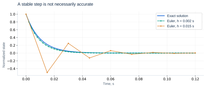
A step of 1.5τ is stable but alternates signs, unlike the exact exponential. For accuracy, use a much smaller step and verify convergence. There is no universal number of points suitable for all problems. Sharp inputs and fast dynamics require particular attention.

Adaptive integration

sol = solve_ivp(motor, (0, 1.5), [0, 0],
                t_eval=np.linspace(0, 1.5, 1501),
                rtol=1e-8, atol=[1e-10, 1e-8],
                max_step=0.005)
assert sol.success, sol.message
current, speed = sol.y

RK45 adapts its internal steps using an estimated local error. t_eval specifies output times, not integration step size. Component-specific absolute tolerances account for different units and scales. The scale atol + rtol·|x| controls local error, not a guaranteed global error.

Switching and events

End an interval exactly at a known load step, preserve its final state and start the next interval with the new input. This prevents a short pulse from falling between internal steps. Use event functions for unknown crossing times, but remember that multiple crossings inside one large step may be missed.

Three independent checks

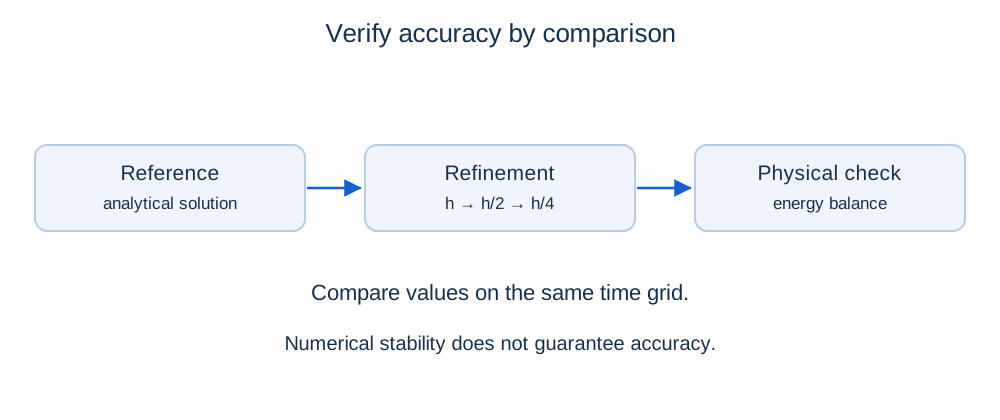
Compare with an analytical RL reference, repeat with smaller steps or tighter tolerances, and verify physical properties: energy, continuity and equilibrium. Agreement between two numerical runs does not prove the model is correct. Large separation between electrical and mechanical time scales can make the problem stiff; compare Radau or BDF with RK45 after checking units and equations.

Euler stability for complex poles

Check every eigenvalue. The base motor’s fast pole −97.407 s⁻¹ gives h < 0.02053 s. At h = 0.02 s its multiplier is about −0.948, so a stable calculation still alternates artificially. Monotonic decay of that mode requires h ≤ 0.01027 s; accurate results usually require smaller steps.

Runge–Kutta and convergence order

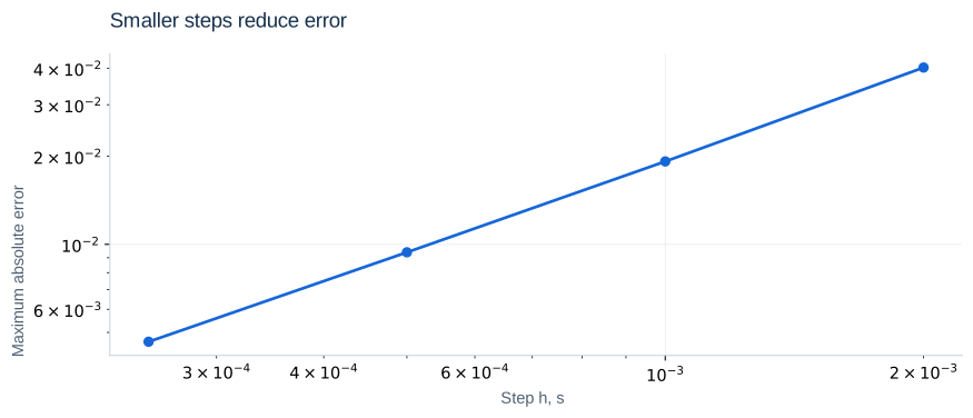
For sufficiently smooth problems on a fixed interval, Euler has global error O(h) and classical RK4 has O(h⁴). A discontinuity within a step violates smoothness; split the interval at known switches. Higher order does not remove explicit-method stability limits on stiff systems.

Measuring convergence

Compare at identical times in the asymptotic convergence range. Roundoff and discontinuities can invalidate the estimate. Do not add amperes and rad/s into an unscaled vector error: normalize components or assess them separately.

Further reading: SciPy: solve_ivp. Notation may differ from this course.

Independent exercises

1. Use Euler for x′ = −10x, x₀ = 1 up to 0.1 s with h = 0.05, 0.025 and 0.0125 s.

2. Find the Euler step limit for λ = −2 + 20j s⁻¹.

Practical work

Solve the RL problem with Euler steps 2, 1, 0.5 and 0.25 ms and plot maximum absolute error against step size. Compare motor solutions at rtol = 10⁻⁵ and 10⁻⁸ on one output grid. Report the method, tolerances, initial conditions, event handling and convergence table.

Calculated illustrations

Key takeaways

Check the model, then numerical stability and accuracy. A dense plotting grid does not imply accurate internal integration.