Braking and reversal
Current, torque and power signs as a drive decelerates or reverses.
Before you begin: the motor equations, power balance and signed quantities.
After this lesson you can: distinguish braking modes, estimate braking time and check consumed and returned energy.
Work through the explanation, examples, practical experiment and independent exercises.
Braking needs a circuit definition
Removing a command, shorting the armature, connecting a braking resistor and reversing the source are different experiments. An ideal source in our model can supply or absorb energy; a real converter may not. Preserve both states across switching and specify how load torque behaves when rotation reverses.
Four mechanical quadrants
Positive speed and positive torque mean forward motoring; positive speed and negative torque mean forward braking. Negative speed and negative torque mean reverse motoring; negative speed and positive torque mean reverse braking. To call braking regenerative, also verify ui < 0 and that the source can accept energy. Electromagnetic braking does not automatically imply electrical energy return.
Current is continuous during reversal
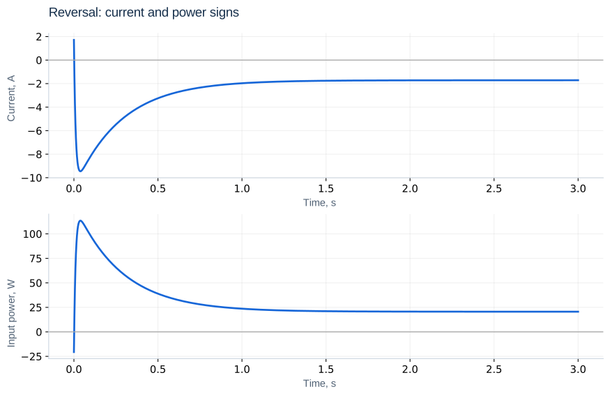
Reversing the voltage does not instantly reverse current or speed. The old current can briefly keep producing the old torque. During plugging, the source may supply energy while the rotor also releases energy, and their sum becomes resistive loss. Keep signs in ui and Meω; absolute values hide the operating mode.
Dynamic braking with a resistor
i ≈ −keω/RΣ; τbrake = J/(b + ktke/RΣ)
Rb ≥ max(0, ke|ω₀|/Ilimit − R)
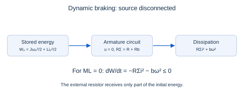
After disconnecting the source, close the armature through Rb. This inequality is an initial quasi-steady sizing estimate, not a substitute for the full transient with nonzero initial current. A larger resistance reduces current and braking torque, so braking is slower.
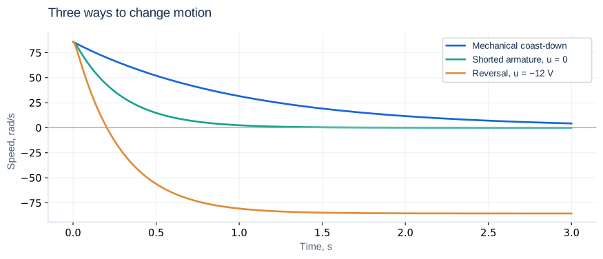
At ω₀ = 80 rad/s and a desired quasi-steady current no larger than 2 A, RΣ ≥ 4 Ω, hence Rb ≥ 2 Ω. With Rb = 2 Ω, τbrake = 0.444 s; reaching 10% speed takes about 1.023 s.
Estimating reversal time
tzero = τeffective ln[(ω₀ − ω∞)/(−ω∞)]
With no external load and symmetrical opposite equilibria, tzero = τeffective ln 2 ≈ 0.198 s. This is a reduced-model estimate. For the full base motor reversing from no-load equilibrium, i₀ = 1.714 A and ω₀ = 85.714 rad/s. Immediately after applying −12 V, current slope is −1200 A/s while acceleration remains initially zero. Braking develops as current changes.
Track both directions of energy
Ereturned = ∫ max(−ui,0) dt
Also integrate armature loss, external resistor loss, viscous loss and load work, and include changes in magnetic and kinetic energy. A net input integral alone hides simultaneous periods of consumption and regeneration. Locate zero crossings of speed, current and power separately.
Independent exercises
1. With Rb = 2 Ω, ω₀ = 80 rad/s, i₀ = 0 and ML = 0, estimate external resistor energy using the full model.
Show solution
Initial energy is 6.4 J. Numerical integration gives about 1.769 J in Rb, 1.769 J in armature R and 2.862 J in viscous friction. Rb receives half the electrical loss, not half the total energy.
2. With ω = 50 rad/s, u = −12 V and steady current, calculate current and powers.
Show solution
i = (−12 − 5)/2 = −8.5 A; ui = +102 W; Meω = −42.5 W; Ri² = 144.5 W. This is plugging: both source and mechanics feed copper losses.
Practical work
Compare dynamic braking and voltage reversal from the same initial state. Plot current, speed, ui and Meω; locate zero crossings and calculate consumed and returned energies separately. Compare full and zero-inductance braking estimates.
Calculated illustrations
Key takeaways
Name the braking circuit and preserve signs. Braking torque, negative speed and regeneration are three different observations.
Progress is stored only in this browser.